Understand how does new pipe work
Include libraries:
1
2
|
library(magrittr)
library(dplyr)
|
1
2
|
##
## Attaching package: 'dplyr'
|
1
2
3
|
## The following objects are masked from 'package:stats':
##
##     filter, lag
|
1
2
3
|
## The following objects are masked from 'package:base':
##
##     intersect, setdiff, setequal, union
|
New pipe |> forces to call function directly while magittr pipe %>% does not need ()
1
2
3
|
abc <-3

abc |> sqrt()
|
One more example.
1
2
3
4
|
mtcars %>%
  select(where(is.numeric)) %>%
  na.omit %>%
  sapply(mean)
|
1
2
3
4
|
##        mpg        cyl       disp         hp       drat         wt       qsec
##  20.090625   6.187500 230.721875 146.687500   3.596563   3.217250  17.848750
##         vs         am       gear       carb
##   0.437500   0.406250   3.687500   2.812500
|
1
2
3
4
|
mtcars |>
  select(where(is.numeric)) |>
  na.omit () |>
  sapply(mean)
|
1
2
3
4
|
##        mpg        cyl       disp         hp       drat         wt       qsec
##  20.090625   6.187500 230.721875 146.687500   3.596563   3.217250  17.848750
##         vs         am       gear       carb
##   0.437500   0.406250   3.687500   2.812500
|
But for some cases |> will not work:
1
2
|
# works
1:10 %>% (call("sum"))
|
1
2
|
# won't work
# 1:10 |> (call("sum"))
|
For lazy typers both of them support lambda syntax. Here is minor differences:
1
2
3
4
|
a <- 10

# regular lambda function
a %>% (function(x) x^2)
|
1
|
a |> (function(x) x^2)()
|
1
2
|
# short one
a %>%  (\(.) .^2)
|
1
2
|
# strange one
a %>% {a^2}
|
1
2
3
4
5
6
7
|
# so, it won't work...
# a |> {a^2}
# a |> {a^2}()

# ... but if you wish so much
.d <- `{`
a |> .d(a^2)
|
Magrittr pipe allows us to use . operator to send the data
1
|
sample(1:10) %>% paste0(LETTERS[.])
|
1
|
## [1] "8H" "1A" "3C" "2B" "9I" "7G" "4D" "5E" "10J" "6F"
|
1
2
|
# This can be avoided:
rnorm(100) %>% {c(min(.), mean(.), max(.))} %>% floor
|
1
2
|
# won't work either
# rnorm(100) |> .d(c(min(.), mean(.), max(.)))
|
Lambda expressions
One example
1
2
3
4
5
|
iris %>%
  {
    size <- sample(1:10, size = 1)
    rbind(head(., size), tail(., size))
  }
|
 1
 2
 3
 4
 5
 6
 7
 8
 9
10
11
12
13
|
##     Sepal.Length Sepal.Width Petal.Length Petal.Width   Species
## 1            5.1         3.5          1.4         0.2    setosa
## 2            4.9         3.0          1.4         0.2    setosa
## 3            4.7         3.2          1.3         0.2    setosa
## 4            4.6         3.1          1.5         0.2    setosa
## 5            5.0         3.6          1.4         0.2    setosa
## 6            5.4         3.9          1.7         0.4    setosa
## 145          6.7         3.3          5.7         2.5 virginica
## 146          6.7         3.0          5.2         2.3 virginica
## 147          6.3         2.5          5.0         1.9 virginica
## 148          6.5         3.0          5.2         2.0 virginica
## 149          6.2         3.4          5.4         2.3 virginica
## 150          5.9         3.0          5.1         1.8 virginica
|
Using . operator re assign data to variable and perform calculations
1
2
3
4
5
6
|
iris %>%
  {
    my_data <- .
    size <- sample(1:10, size = 1)
    rbind(head(my_data, size), tail(my_data, size))
  }
|
 1
 2
 3
 4
 5
 6
 7
 8
 9
10
11
12
13
14
15
|
##     Sepal.Length Sepal.Width Petal.Length Petal.Width   Species
## 1            5.1         3.5          1.4         0.2    setosa
## 2            4.9         3.0          1.4         0.2    setosa
## 3            4.7         3.2          1.3         0.2    setosa
## 4            4.6         3.1          1.5         0.2    setosa
## 5            5.0         3.6          1.4         0.2    setosa
## 6            5.4         3.9          1.7         0.4    setosa
## 7            4.6         3.4          1.4         0.3    setosa
## 144          6.8         3.2          5.9         2.3 virginica
## 145          6.7         3.3          5.7         2.5 virginica
## 146          6.7         3.0          5.2         2.3 virginica
## 147          6.3         2.5          5.0         1.9 virginica
## 148          6.5         3.0          5.2         2.0 virginica
## 149          6.2         3.4          5.4         2.3 virginica
## 150          5.9         3.0          5.1         1.8 virginica
|
Building unary functions with %>%
1
2
3
4
5
|
trig_fest <- . %>% tan %>% cos %>% sin

one2ten <- 1:10

one2ten %>% trig_fest
|
1
2
|
##  [1]  0.0133878 -0.5449592  0.8359477  0.3906486 -0.8257855  0.8180174
##  [7]  0.6001744  0.7640323  0.7829771  0.7153150
|
1
2
|
# same as:
sin(cos(tan(1:10)))
|
1
2
|
##  [1]  0.0133878 -0.5449592  0.8359477  0.3906486 -0.8257855  0.8180174
##  [7]  0.6001744  0.7640323  0.7829771  0.7153150
|
1
2
|
# or:
one2ten |> trig_fest()
|
1
2
|
##  [1]  0.0133878 -0.5449592  0.8359477  0.3906486 -0.8257855  0.8180174
##  [7]  0.6001744  0.7640323  0.7829771  0.7153150
|
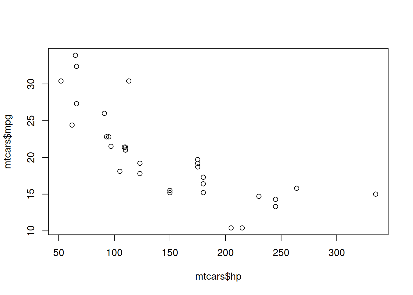
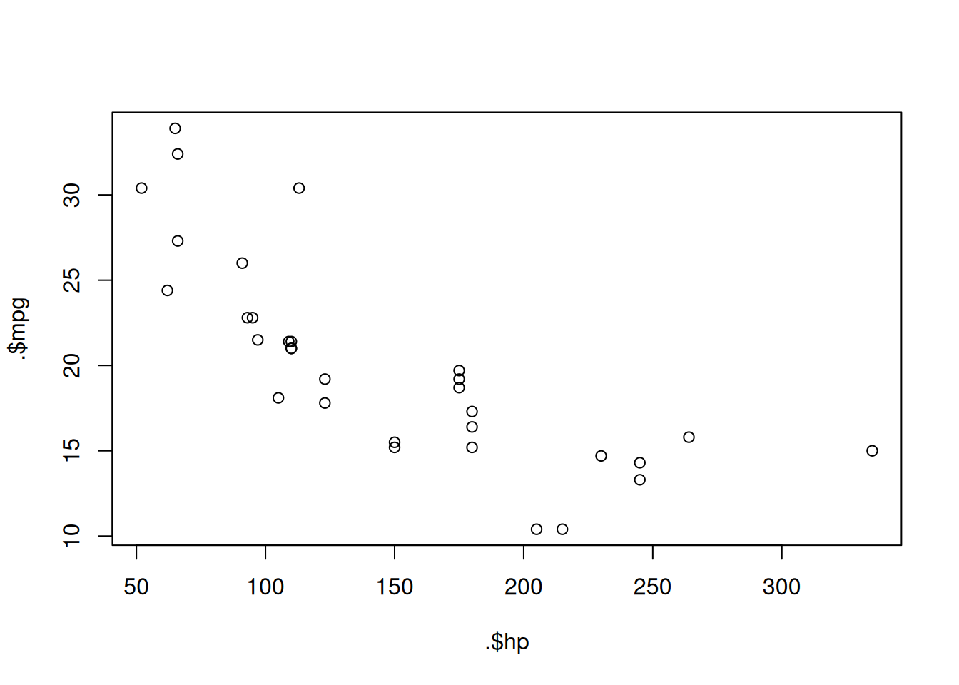
How to send more than one argument into function with pipe?
1
2
|
# normal way
plot(mtcars$hp, mtcars$mpg)
|
1
|
lm(mtcars$mpg ~ mtcars$hp)
|
1
2
3
4
5
6
7
|
##
## Call:
## lm(formula = mtcars$mpg ~ mtcars$hp)
##
## Coefficients:
## (Intercept)    mtcars$hp
##    30.09886     -0.06823
|
1
2
|
# or
lm(mpg ~ hp, data = mtcars)
|
1
2
3
4
5
6
7
|
##
## Call:
## lm(formula = mpg ~ hp, data = mtcars)
##
## Coefficients:
## (Intercept)           hp
##    30.09886     -0.06823
|
1
2
3
|
# magrittr pipe way if function has data argument
mtcars %>%
  lm(mpg ~ hp, data = .)
|
1
2
3
4
5
6
7
|
##
## Call:
## lm(formula = mpg ~ hp, data = .)
##
## Coefficients:
## (Intercept)           hp
##    30.09886     -0.06823
|
1
2
3
4
5
|
# but this won't work
# mtcars %>% plot(.$mpg, mtcars$hp)

# but we can override the defaulter behavior using `{` function
mtcars %>% {plot(.$mpg, .$hp)}
|
1
2
3
4
5
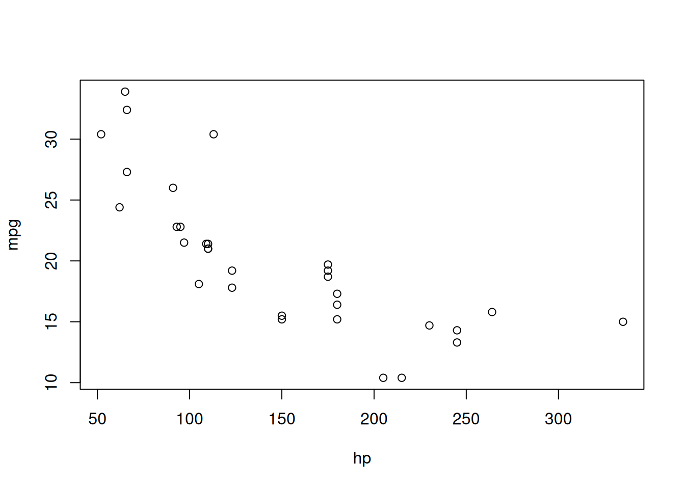
|
# or use with function
with(mtcars, plot(hp, mpg))

# another solution:
mtcars |> with(plot(hp, mpg))
|
1
2
|
# true hacker way
mtcars %$% lm(mpg ~ hp + disp)
|
1
2
3
4
5
6
7
|
##
## Call:
## lm(formula = mpg ~ hp + disp)
##
## Coefficients:
## (Intercept)           hp         disp
##    30.73590     -0.02484     -0.03035
|
A couple more lambda examples from new 4.1 R update.
1
2
3
|
# the shortcut for anonymous functions \(x) {} is the same as function(x) {}:

mtcars |> (\(x) {x[which.max(x$mpg), ]})()
|
1
2
|
##                 mpg cyl disp hp drat    wt qsec vs am gear carb
## Toyota Corolla 33.9   4 71.1 65 4.22 1.835 19.9  1  1    4    1
|
1
|
mtcars |> (\(.) {.[which.max(.$mpg), ]})()
|
1
2
|
##                 mpg cyl disp hp drat    wt qsec vs am gear carb
## Toyota Corolla 33.9   4 71.1 65 4.22 1.835 19.9  1  1    4    1
|
1
2
3
|
# Curly bracets for the first expression, {}(), work too:

mtcars |> {\(x) {x[which.max(x$mpg), ]}}()
|
1
2
|
##                 mpg cyl disp hp drat    wt qsec vs am gear carb
## Toyota Corolla 33.9   4 71.1 65 4.22 1.835 19.9  1  1    4    1
|
1
2
3
|
# same as

mtcars %>% (\(.) {.[which.max(.$mpg), ]})
|
1
2
|
##                 mpg cyl disp hp drat    wt qsec vs am gear carb
## Toyota Corolla 33.9   4 71.1 65 4.22 1.835 19.9  1  1    4    1
|
1
2
3
|
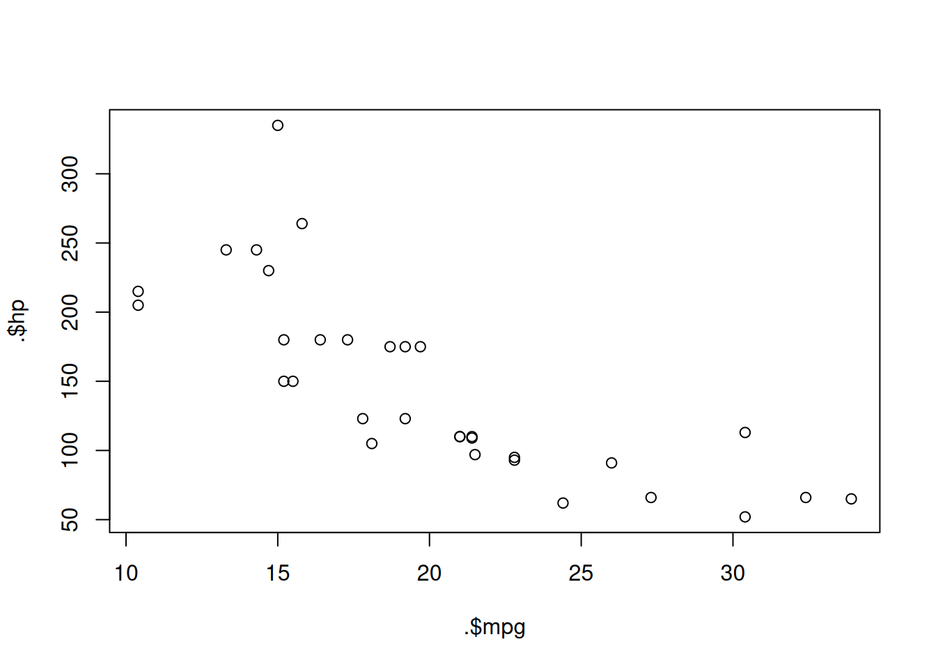
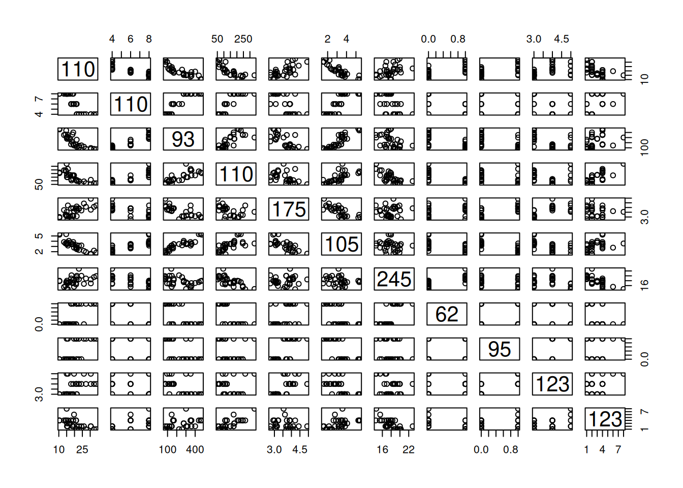
# lets plot

mtcars %>% plot(.$hp)
|
 1
 2
 3
 4
 5
 6
 7
 8
 9
10
|
# won't work
# mtcars |> plot(.$hp) # error
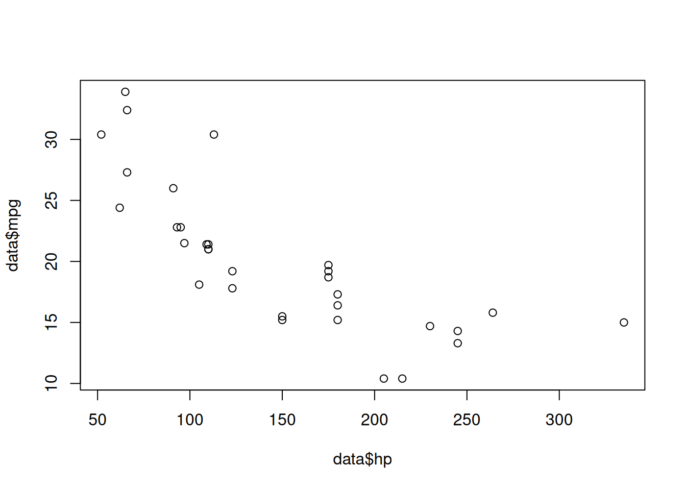
# Getting to the solution
# verbosely
mtcars |> (function(.) plot(.$hp, .$mpg))()
# using the anonymous function shortcut for emulation the dot syntax
mtcars |> (\(.) plot(.$hp, .$mpg))()
|
1
2
|
# or more readable
mtcars |> (\(data) plot(data$hp, data$mpg))()
|